Experiment Configuration

NXRefine uses a hierarchical directory structure for each experiment to store both the raw data generated on an x-ray beamline and processed data generated by the data reduction workflow. An ‘experiment’ in NXRefine comprises measurements on a set of samples that are logically grouped together, often because they are performed within a specific time period and/or share calibration files. Plugins to the NeXpy GUI are used to facilitate the creation of both the directory hierarchy and the associated data files.

Data that are processed by the NXRefine package are stored as HDF5 files that conform to the NeXus format, which is an international standard for the storage of x-ray and neutron scattering data. There is a single NeXus file associated with each measurement, which consists of one or more rotation scans usually at a single temperature or other parametric variable. This file contains all the information required for a complete analysis, including external links to the raw data, beamline monitors, powder diffaction calibrations, and metadata generated by the data reduction workflow.

In this section, we will describe the NXRefine directory framework, explaining where the NeXus files are stored and how they are linked to the reduced data transformed into reciprocal space. At the beginning of each new experiment, the GUI dialogs launched from the Experiment Menu can be used to create the experiment directories, NeXus file templates, and new NeXus files based on those templates to contain scan data.

Experiment Layout

In NXRefine, it is assumed that all the files associated with a particular experiment are stored in a single directory. At synchrotron x-ray facilities, it is common to schedule all the measurements associated with a particular proposal together, associated with a proposal number and/or run cycle. For example, on beamline 6-ID-D at the Advanced Photon Source, measurements resulting from Proposal No. GUP-75969 may be scheduled in a specific run cycle, say 23-1, and stored in, e.g., /data/6-id-d/GUP-75969-23-1. This directory should contain sub-directories that conform to a particular layout, with calibration files stored in the directory calibrations, NeXus files containing measurement templates stored in configurations, settings and log files stored in tasks, and experimental data from each sample stored in separate directories with a name that is typically derived from the chemical formula or a commonly used abbreviation. It is common to test and/or measure multiple crystals with the same chemical formula, so each of the sample directories contain sub-directories for each measured crystal. These contain the NeXus files for each scan and linked sub-directories containing the raw data.

Here is the structure of a possible experiment directory. Most of the names in this example are chosen to be generic, i.e., they will be different for every experiment. The only exceptions are the files in the tasks directory, which are set automatically by NXRefine.:

experiment
└── tasks
    ├── nxdatabase.db
    ├── nxlogger.log
    ├── settings.ini
└── calibrations
    └── powder_calibration.tiff
└── configurations
    ├── configuration.nxs
└── sample1
    └── label1
        ├── sample1_100K.nxs
        └── 100K
            ├── f1.h5
            ├── f2.h5
            ├── f3.h5
            ├── f1_transform.nxs
            ├── f2_transform.nxs
            ├── f3_transform.nxs
            └── transform.nxs
        ├── sample1_200K.nxs
        └── 200K
            ├── ...
        └── sample1_300K.nxs
        └── 300K
            ├── ...
    └── label2
        └── sample1_300K.nxs
        └── 300K
            ├── ...
├── sample2
├── sample3

The goal of this directory structure is for all the data and metadata required to analyze the results to be stored in an easily accessible location, although not all files are required by NXRefine to be present. For example, the powder calibration files can be imported from any location.

If an instrument does not exclusively use NXRefine for its data reduction, it is possible that an experiment directory already exists. If so, in order to avoid any interference with other instrument files, it is possible to create the above directory structure within a sub-directory, called nxrefine, contained within the existing experiment directory.:

experiment
└── nxrefine
    ├── tasks
    ├── calibrations
    ├── configurations
    ├── scripts
    ├── sample1
    └── sample2
    .
    .
    .

Note

The name of this sub-directory is defined in the server settings, which are described below. It is strongly recommended that it be called by the default name, i.e., nxrefine to facilitate parsing of the directory tree.

Experiment Sub-Directories

tasks

The tasks sub-directory contains a number of files used by NXRefine to store default settings, workflow logs, and a MySQL database for recording the status of each workflow component. The files in this directory are created automatically by NXRefine and should not be touched. NeXpy GUIs are used to inspect their contents.

calibrations

The calibrations sub-directory is designed to contain either the TIFF or CBF files generated by measurements of a calibrant powder, or a file, usually with extension .poni, containing the instrument parameters calibrated using the PyFAI module. The workflow includes a GUI for performing PyFAI calibrations directly on powder calibration image files, with the results stored in the NeXus files (described below). The files don’t have to be stored in this sub-directory, but if they are in another location, it is recommended to copy them here for completeness. If the calibrations have been performed by another package, the parameters can be imported directly from a PONI file.

configurations

The configurations sub-directory contains NeXus files that act as templates to be used when creating the files used to store the scan results. There should be a separate template file for each new experimental configuration, .e.g., with a different wavelength or detector distance. If multiple sample rotations are to be performed with different detector translations and/or goniometer angles, the corresponding template files will have entries for each scan containing pre-defined values of the scan variables. These files are initialized by a NeXpy GUI dialog.

Note

On QM2 at CHESS, it is usually only necessary to create template files with a single entry, since the number of rotation scans is not always pre-determined. When the scans are imported, additional entries are automatically added with the goniometer angles updated with the values in the corresponding scan SPEC file.

scripts

The scripts sub-directory is not used directly by NXRefine, but is created by the New Experiment dialog described below. It is designed to store macros for use during an experiment.

sample

The sample sub-directories are typically named after a common abbreviation or chemical formula of the measured sample (e.g., TiSe2). Within each sample directory are one or more directories usually corresponding to different crystals, specified by unique labels typically provided by the crystal grower. It is common in these experiments to screen a number of crystals before selecting one for further measurements, in which case many of these directories would only contain a single scan.

Within each label directory, there are one or more directories that are named after the parametric variable being modified between each set of rotation scans, e.g., 100K. These scan directories contain the raw data in HDF5 files, typically with extension .h5. Each one of these .h5 files contain the raw data from a single rotation scan stacked into a single HDF5 array. It is common to perform three sample rotations, which are then stored in f1.h5, f2.h5, and f3.h5, but any number is possible. The scan directories also contain other files produced during the data reduction procedure, such as data transformed into reciprocal space coordinates or pair-distribution functions.

For each of these scan directories, there is a corresponding NeXus file that is named as, e.g., sample_scan.nxs, where sample must be the name of the sample directory and scan should be the name of the directory containing the raw data. These NeXus files contain external links to the much larger files stored in the scan directories. By opening them, the user has access to all the data and metadata associated with a particular scan, since external links, if they are available, will appear to be part of the file.

Note

External links are defined by the file name and internal path to the required HDF5 field. If the file and/or field are not available, the NeXus file can still be opened, but the corresponding data cannot be viewed. The file name is stored as a relative file path, so the NeXus file and a subset of the files in the scan directory can be moved to another location if, for example, access to the raw data is no longer necessary.

Instrument Setup

The experiment directory layout can be created automatically using GUI dialogs in the NeXpy “Experiment” menu. Before using them, it is important to have initialized the default instrument parameters using the “Edit Settings” dialog of the NeXpy “Server” menu, or at the command line using nxsettings -i.

The instrument settings provide information on the directories, in which both the raw data and the NXRefine directory tree are located. It is quite common for the raw data to be collected as a set of image files, typically TIFF or CBF files. These are usually not stored in the experiment directories described in the previous section, and may be in read-only directories. To allow for the input of such files, NXRefine defines two sets of paths; one to the ‘raw’ data and one to the NXRefine (or ‘analysis’) directories. It is assumed that the experiment names, e.g., GUP-75969-23-1, are the same in both locations, although alternative methods of linking the ‘raw’ and ‘analysis’ paths could be defined in the customized beamline classes described later.

For example, at CHESS, the ‘raw’ and ‘analysis’ paths are defined in parallel directory trees as follows (with generic experiment names):

/nfs/chess/id4b                         /nfs/chess/id4baux
├── 2023-1                              ├── 2023-1
├── 2023-2                              ├── 2023-2
└── 2023-2                              └── 2023-2
    ├── experiment1                         ├── experiment1
    ├── experiment2                         ├── experiment2
    └── experiment3                         └── experiment3
        └── raw6M                               └── nxrefine
            ├── sample1                             ├── sample1
            ├── sample2                             ├── sample2
            └── sample3                             └── sample3
                └── label1                              └── label1
                    ├── 100                                 ├── 100
                    ├── 200                                 ├── 200
                    └── 300                                 └── 300

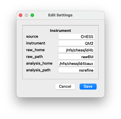
Here is a list of instrument parameters.

source

This is the name of the synchrotron source, at which the instrument is located. This will be stored in the NeXus files during the data reduction, but is not otherwise used.

instrument

This is the name of the instrument. If a customized beamline package is to be imported, this must correspond to the instrument name used in the package.

raw_home

This is the home directory, in which the experimental raw data are stored. In the above example, this could be /nfs/chess/id4b/2023-3.

raw_path

This is the path within the experiment directory to the sample directories. In the above example, this would be raw6M.

analysis_home

This is the home directory, in which the data are analyzed. In the above example, this could be /nfs/chess/id4baux/2023-3.

analysis_path

This is the path within the experiment directory to the NXRefine sub-directories. In the above example, this would be nxrefine.

On Sector 6 at the APS, the images are automatically stacked as HDF5 files and saved in the analysis directories as f1.h5, f2.h5, etc, so the paths to the raw data are not required and can be left blank. The ‘analysis_path’ field is also blank, since the sample directories are at the top level of the experiment directories.

If someone wants to use NXRefine to analyze data collected as image files, which are not stored in a directory tree compatible with the above description, there are two options. Firstly, the NXBeamLine class, which is described later, is designed to allow beamline-specific methods of importing the data and metadata. These can be implemented in separate packages that are imported into NXRefine as plugins. Secondly, the image files can be loaded into HDF5 files using the nexusformat command-line script, ‘nxstack’ and saved to the scan directories described above. Type nxstack -h at the terminal command line to see possible options.

Experiment Menu

The NXRefine plugin to NeXpy installs a top-level menu labelled “Experiment”. The sub-menus run operations to initialize the experiment layout, create experimental data templates, calibrate powder data, and initialize new data files.

New Experiment

This dialog initializes a new experiment directory layout using the server settings to initialize default locations. When the dialog is launched, click on “Choose Experiment Directory” to launch the system file browser in order to select or create the new experiment directory.

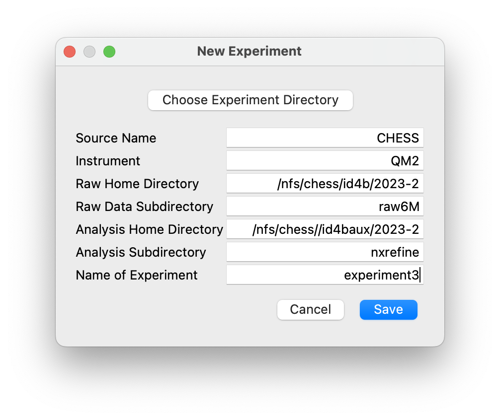
There are two scenarios.

1. If raw_home is not blank in the server settings, the file browser will default to the raw_home directory, in which an experiment directory, containing the raw image files, should already exist. This experiment directory is then selected, after which the dialog above is created, with the experiment name (i.e., the base name of the experiment directory path) already filled in, along with the path to analysis home directory (analysis_home in the server settings) and the name of the analysis sub-directory if required. When the “Save” button is pressed, the new experiment directory is created within the analysis home directory if it does not already exist, and the experiment directory tree is initialized with the calibrations, configurations, scripts and tasks sub-directories.

2. If raw_home is blank, the file browser will default to the analysis_home directory, but another location can be selected if required. The file browser can be used either to select an existing experiment directory or to create a new one. The above dialog is then created with the experiment name given by the base name of the selected experiment directory path, and the analysis home directory defined by its parent. When the “Save” button is pressed, the experiment directory tree is initialized with the calibrations, configurations, scripts and tasks sub-directories.

A new settings.ini file is created in the tasks sub-directory, with values copied from the equivalent file in the server directory, excluding the “Server” section. This allows the refinement parameters to be customized for each experiment.

New configuration

This dialog creates NeXus files that are used as templates for the experimental files that are used to store all the data and metadata associated with a particular set of rotation scans. The initial metadata is defined by parameters in the settings file in the tasks sub-directory, which can be modified by the “Edit Settings” sub-menu described below. However, some of the metadata will be refined using a powder calibration, whose results are then stored in this file.

After selecting the experiment directory, the following dialog is created.

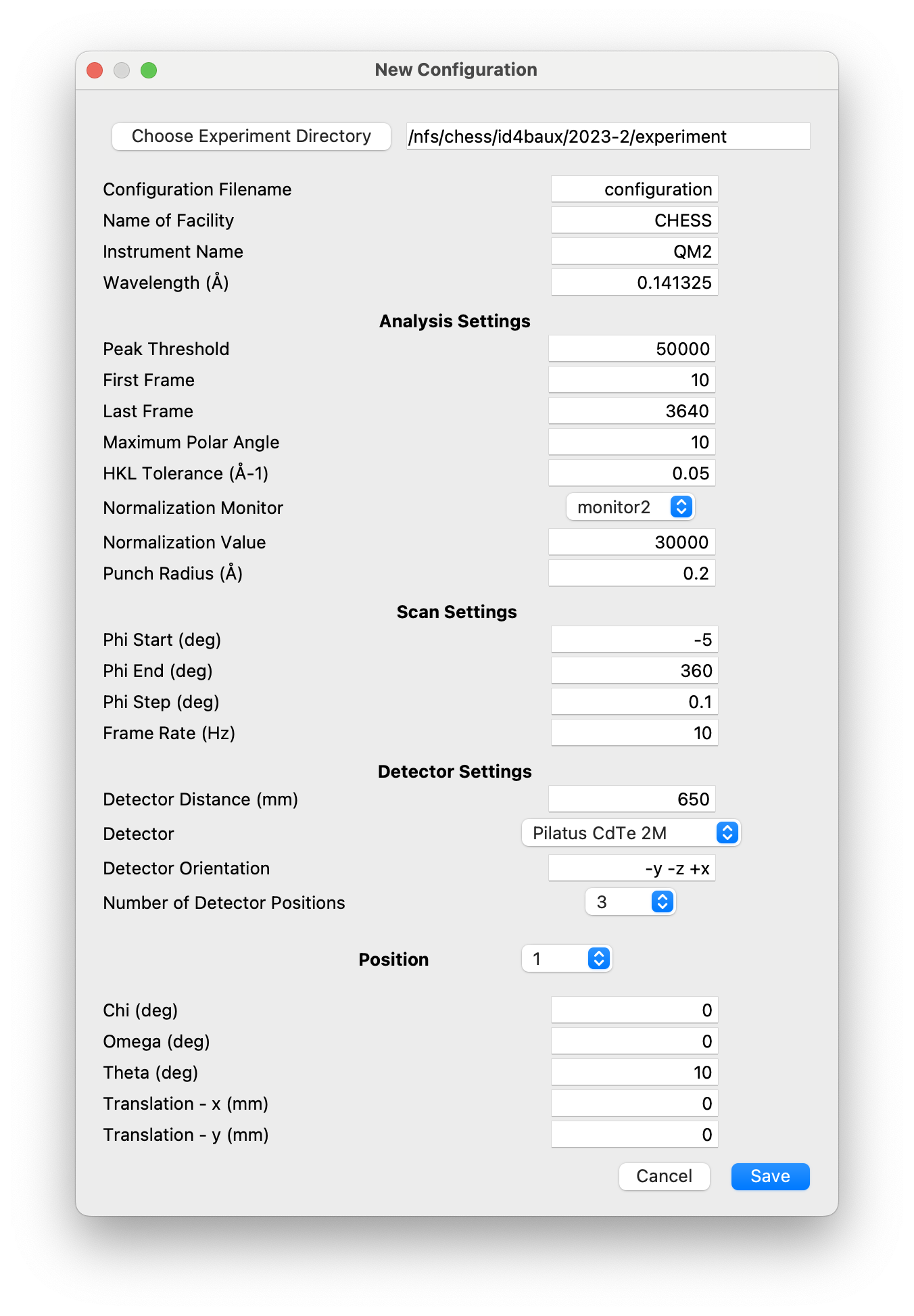
This allows the settings used in subsequent analysis to be initialized, the parameters defining the rotation scans (range, step size, frame rate) to be set, the detector configuration to be defined, and the angles and/or detector positions to be used in one or more rotation scans. These are all saved to the NeXus template. The wavelength and detector distance can be nominal values at this stage, since they are updated by performing a powder calibration. Similarly, the instrument angles, \(\theta\), \(\omega\), and \(\chi\) are set to the angles set by the motors, but will usually be refined when the sample orientation is determined.

It is possible to create more than one configuration template, if, for example, different angles and/or detector positions are used in different phases of an experiment. NXRefine allows the appropriate template to be selected when setting up the scan. A separate template should be created for each configuration that requires a change in the instrument calibration (wavelength, detector distance, detector translation) or scan angles.

The detector is chosen from a pull-down menu that contains all the detectors defined in the PyFAI package. This defines the number of pixels, their size, and a mask array used to exclude all the pixels within gaps between the detector chips.

Calibrate Powder

This dialog will import a TIFF or CBF file containing measurements of a powder calibrant and refine the detector position and coordinates, using the PyFAI API. Alternatively, if the calibration parameters are already available in a PONI file, they can be directly imported. The resulting powder data and calbration parameters are then saved to the configuration template previously created using the New Configuration dialog.

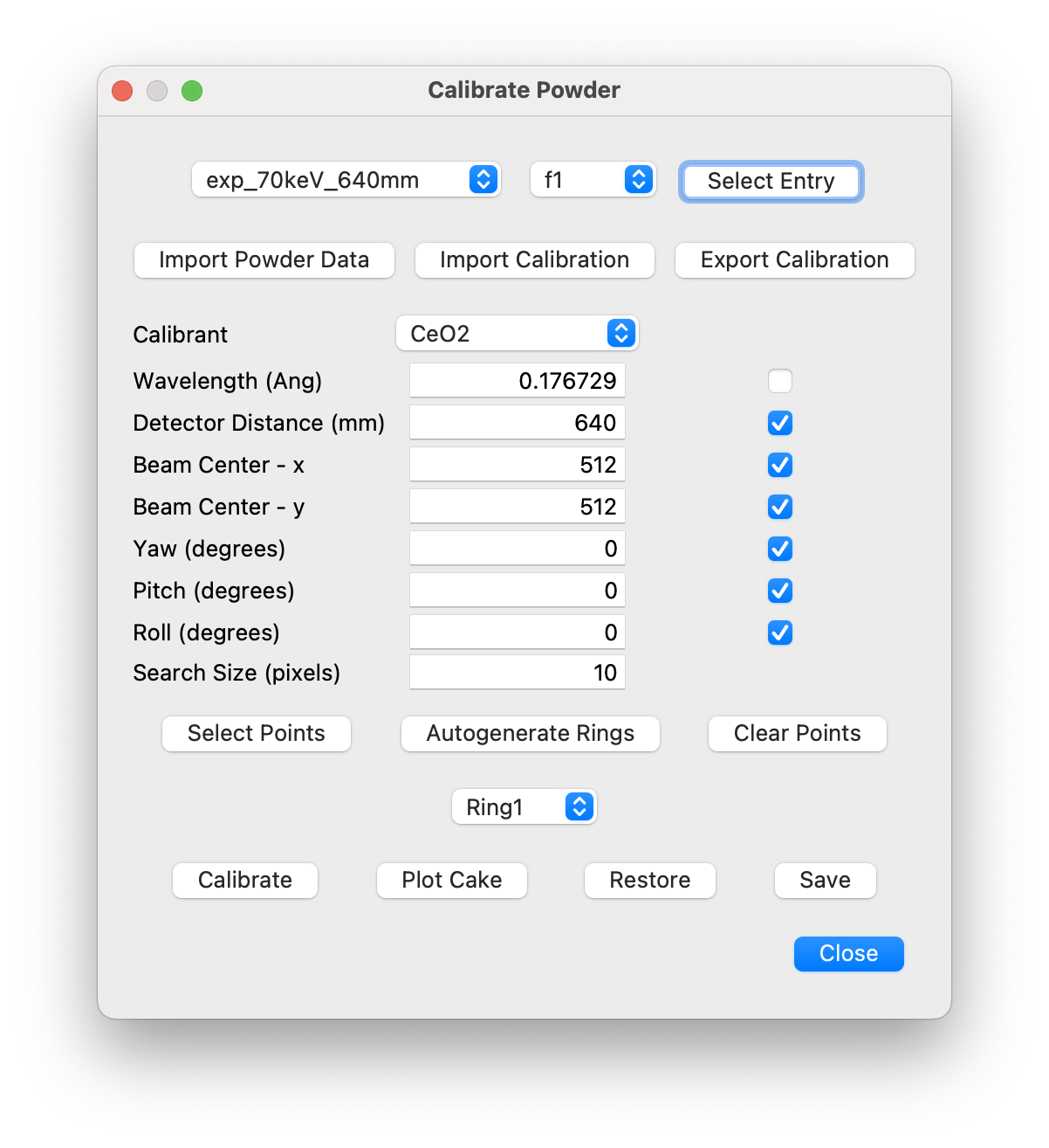
After launching the dialog, select the entry in the configuration file to be calibrated by the powder measurement, i.e., the one with the correct wavelength, detector distance and translations. This expands the dialog with the default parameters defined by the settings file. The checkboxes at the side of each parameter specify whether the parameter is to be refined. By default, the wavelength checkbox is de-selected, since this is normally defined accurately by other means. It is too highly correlated to the detector distance for both to be refined simultaneously.

Then click on “Import Powder Data” to select the powder calibration file. This will generate a plot containing the powder data on a log scale. Select the approprate powder calibrant from those specified in the Calibrant pull-down menu.

If a PONI file already exists from a prior calibration, it can be imported using the “Import Calibration” button. If this is sufficiently accurate, it is not necessary to perform further calibrations. Instead the calibration parameters can be saved to the configuration file by clicking on “Save” and the dialog can be closed.

To obtain an initial calibration, zoom into this plot to display the first few rings.

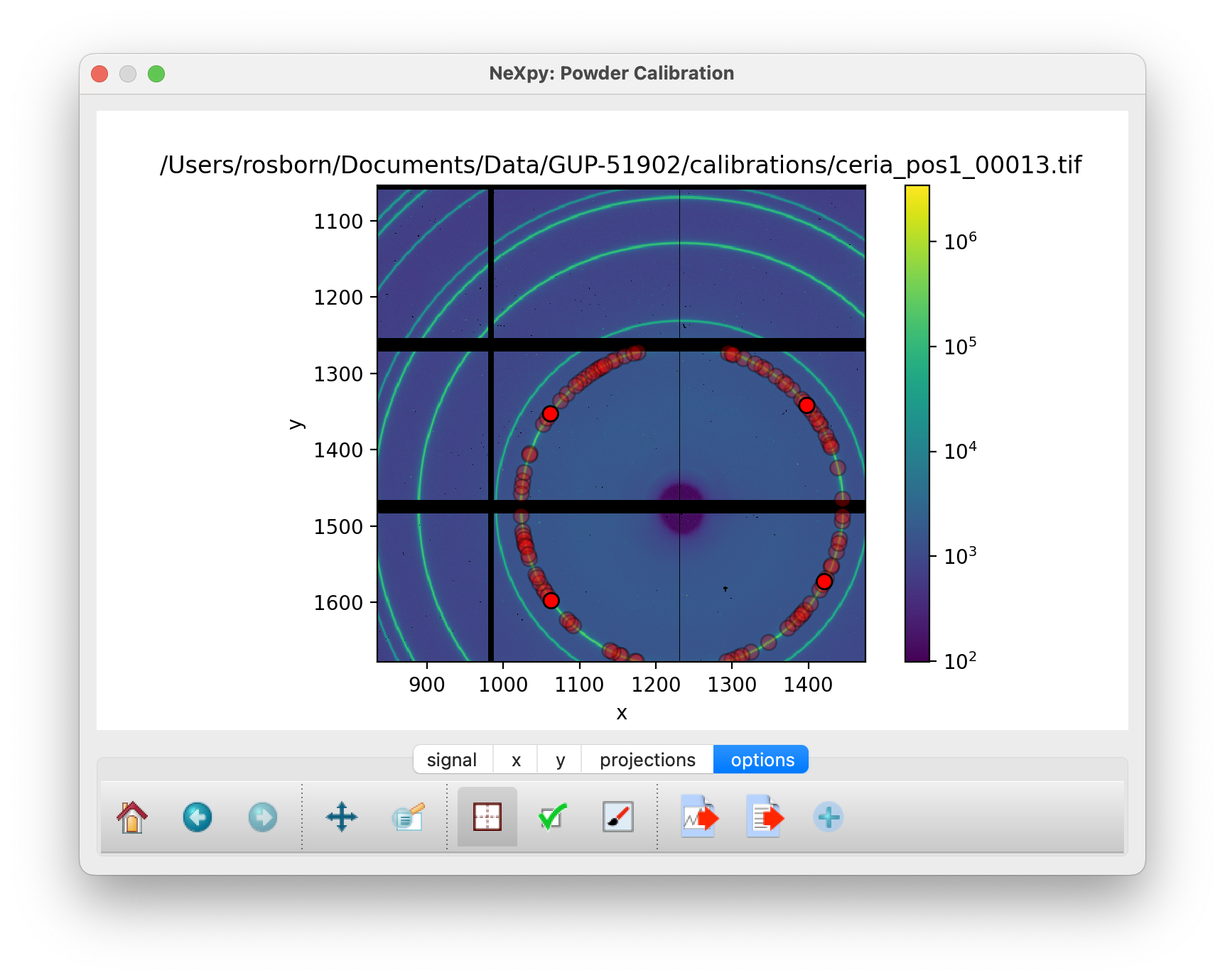
Points generated for the innermost ring after manually selecting four points

After clicking on “Select Points”, click somewhere on the innermost ring. This triggers the PyFAI Massif module, which automatically detects other points on the Debye-Scherrer ring that are contiguous to the selected point. Because of the gaps between detector chips, the Massif detection is confined to pixels within a single chip, so it is normally necessary to select other points on neighboring chips to complete a single ring. In the above ring, four selections, corresponding to the brighter red circles, were made.

It is only necessary to do this for a single ring. De-select the “Select Points” button and click “Calibrate” to perform an initial calibration. After this, it is possible to generate points automatically on the other rings using the “Autogenerate Rings” button. Select how many rings to generate, using the ring pull-down menu.

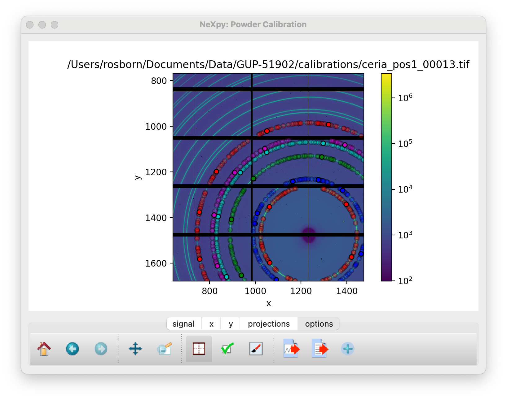
Autogenerated rings after selecting “Ring6” on the pull-down menu

When enough rings have been defined, click “Calibrate” again to produce a more accurate refinement.

The “Plot Cake” button can be used to generate a “cake” plot, in which all the powder rings, which are plotted against polar angle, should fall on vertical lines.

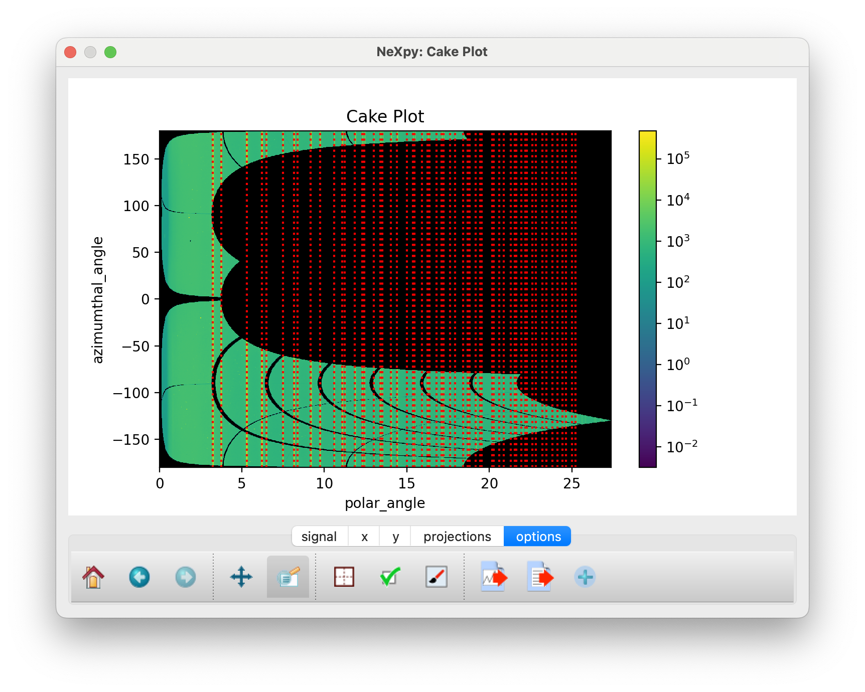
Cake Plot which allows a comparison of the powder data, plotted as a function of polar angle, with the theoretical powder lines (dotted red lines).

This can be used to determine whether the calibration is sufficiently good over the entire angular range of the detector. If there is evidence of distortions at higher polar angle, it may be necessary to autogenerate more rings before an additional calibration.

When the calibration is satisfactory, click “Save” to save both the powder calibration data and parameters to the configuration file. The calibration parameters can also be saved to a PONI file, using the “Export Calibration” button. This process should be repeated for each entry, after which the dialog can be closed.

Create Mask

This dialog creates a pixel mask that is used to exclude bad pixels from further analysis. As described above, when a new configuration file is created, a pixel mask that excludes gaps between detector chips is automatically added. Additional pixels can be excluded using this dialog, either by adding editable shapes that are constructively added to the existing mask or by importing the mask from an external file, which can store the mask in any image format. The latter is useful if a beamline regularly updates a particular detector’s mask as bad pixels are identified.

Warning

If an external mask is input using “Import Mask”, it will overwrite the existing mask. It is important therefore that the external pixel mask also excludes the detector gaps.

After launching the dialog, the current mask is automatically plotted, as an overlay on the powder diffraction data to enable the center of the beam and other features of the data to be identified.

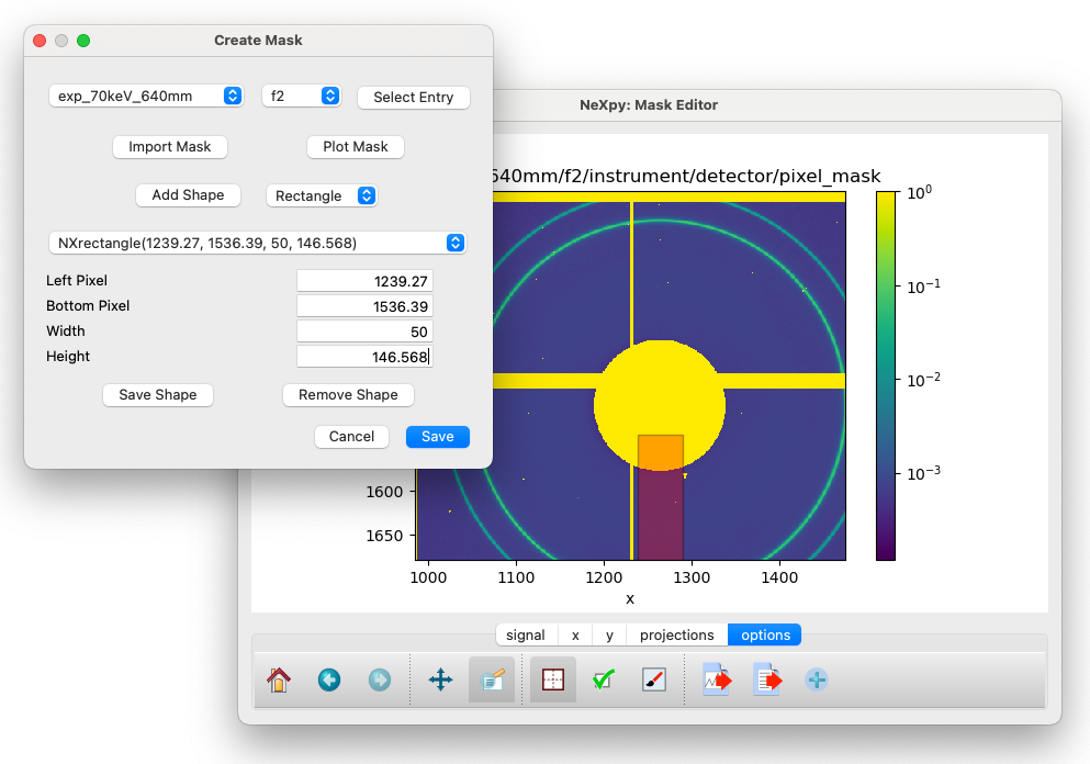
Create Mask dialog. The translucent shape shows the rectangle created by clicking “Add Shape”.

By clicking on “Add Shape” with either a rectangle or circle selected, a translucent shape is added to the plot. By default, it is centered on the beam center, but may be moved by dragging the center of the shape and/or resized by dragging one of the shape edges. When the shape has the correct position and size, click on “Save Shape” for the shape to be added to the current list. A pull-down menu allows existing shapes to be selected for further edits or removal

Note

After saving the shape, it is no longer draggable. However, the shape can still be modified by adjusting the shape parameters and then clicking on “Save Shape” again.

If a more complicated mask is required, it can be generated by an external image editor and imported using “Import Mask”.

When the mask is complete, click “Save” to save it to the configuration file.

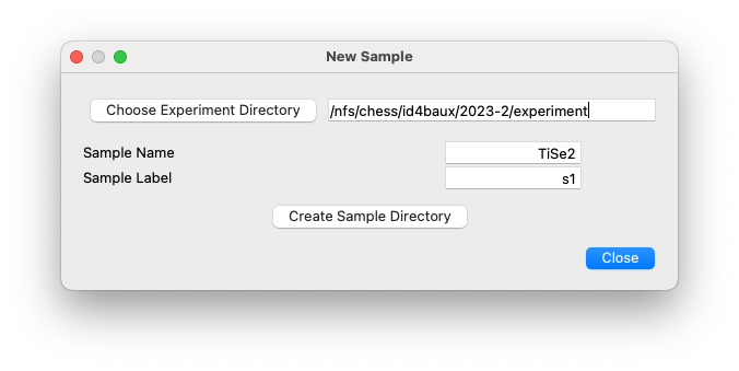
New Sample

This dialog has the single purpose of creating a directory tree for a new sample. The dialog enables the creation of a sample directory within the requested experiment directory and a sub-directory with a unique label for each instance of that sample measured during an experiment.

New Scan

This dialog is used to create a NeXus file in preparation for an experimental measurement. The file will be based on the selected configuration file and be saved in the specified sample/label directory. The name of the file will be “<sample>_<scan>.nxs”, where <scan> is the Scan Label specified in the dialog (‘300K’ in the image below).

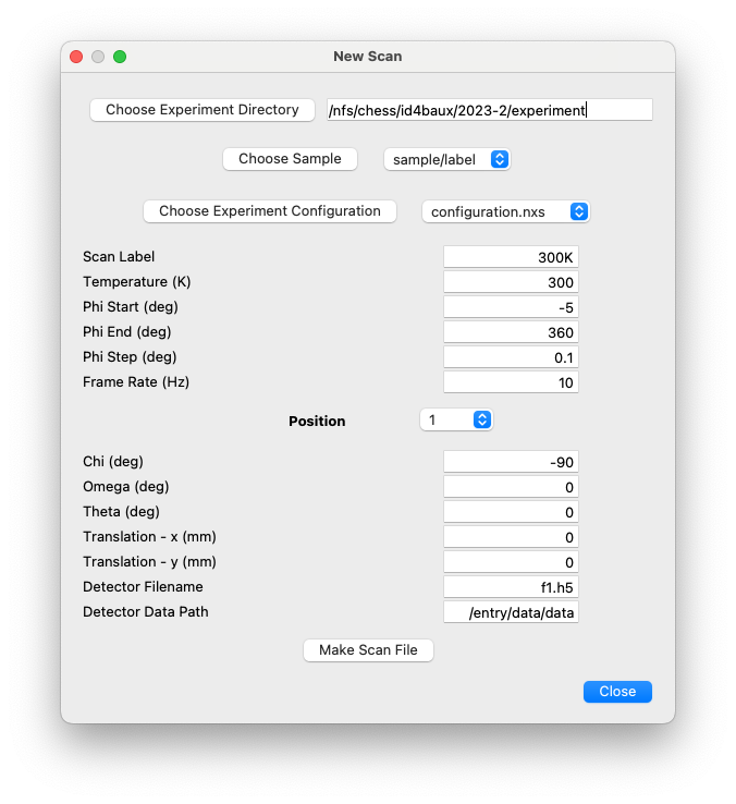
The NeXus file is left open in the NeXpy tree. Multiple files can be created within the dialog, with different scan labels and, typically, different temperatures, before the dialog is closed.

External links to the raw data file are created in the NeXus file, even if the data does not yet exist. In the example above, the external link for the first detector position will be to f1.h5, in the <scan> subdirectory. Similarly, the external link for the second detector position would be to <scan>/f2.h5, etc. This experimental layout is described in more detail in the Experiment Layout section above.

Import Scans

This dialog is for instruments in which the scans are already defined using different methods to those above. For example, on the QM2 instrument at CHESS, the scans are defined in SPEC files, with the data stored separately in a separate read-only directory. With this dialog, the directories containing the raw images are associated with the corresponding SPEC scan, allowing NeXus files to be automatically generated. This customization is encoded in a QM2 sub-class of the NXBeamLine class, which is installed separately as a NXRefine plugin. The process for customizing other beamlines is described later.

Sum Scans

This dialog allows data in NeXus files collected under identical conditions to be summed to produce a single NeXus file that can be processed using the usual workflow.

Edit Settings

This dialog allows the settings, whose default values are defined in the server directory (see Default Settings), to be customized for the data reduction performed in the selected experiment. The settings are stored in <experiment>/tasks/settings.ini. The meanings of each setting are described in the next section.