Introduction

NXRefine implements a complete workflow for both data acquisition and reduction of single crystal x-ray scattering collected by the sample rotation method. The package generates a three-dimensional mesh of scattering intensity, i.e., S(Q), which can be used either to model diffuse scattering in reciprocal space or to transform the data to produce three-dimensional pair-distribution-functions (PDF), which represent the summed probabilities of all possible interatomic vectors in real space, i.e., Patterson maps. If the Bragg peaks are eliminated before these transforms, using a process known as ‘punch-and-fill,’ only those probabilities that deviate from the average crystalline structure are retained. The final stage of the NXRefine workflow is to generate such 3D-ΔPDF maps.

The uncompressed raw data from such measurements comprise tens, and sometimes hundreds, of gigabytes, which can be collected in under 30 minutes. The speed of data collection allows such measurements to be repeated multiple times as a function of a parametric variable, such as temperature. Such data needs to be transformed into reciprocal space as quickly as it is measured, so that scientists can inspect the results before a set of scans is complete. For this reason, the NXRefine workflow is designed to be run automatically once an initial refinement of the sample orientation has been determined.

NXRefine is currently in use on Sector 6-ID-D at the Advanced Photon Source and the QM2 beamline at CHESS, and is under active development at other facilities.

Experimental Geometry

NXRefine is designed for experiments, in which the sample is placed in a monochromatic x-ray beam and rotated continuously about an axis that is approximately perpendicular to the beam. Images are collected on an area detector placed in transmission geometry behind the sample. Many area detectors consist of a set of chips with small gaps between them, so sample rotation scans are often repeated multiple times (typically three) to fill in the missing data, with small detector translations between each scan and/or changes to the orientation of the rotation axis. NXRefine reduces the data independently for each rotation scan before merging them to create a single 3D data volume.

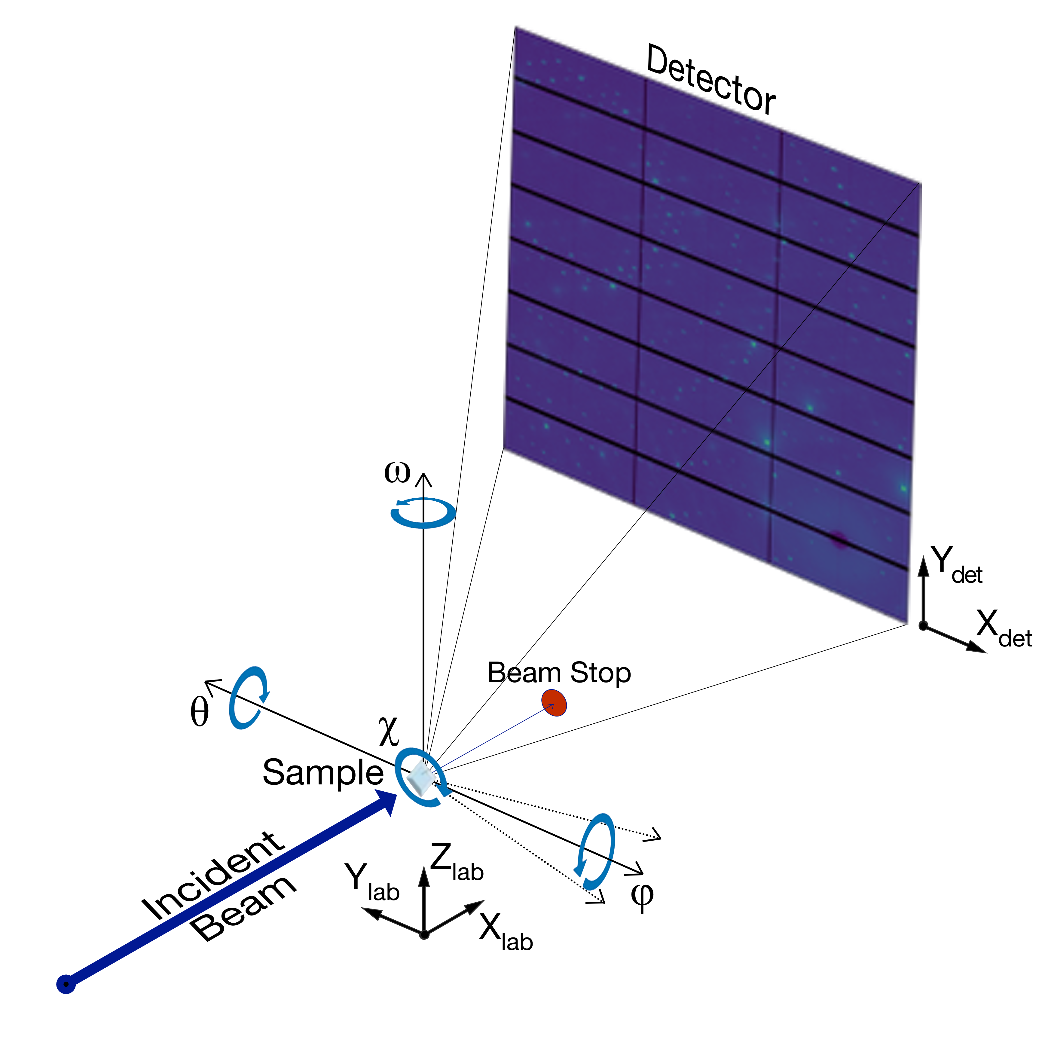
Example of the experimental geometry used in NXRefine, with the Φ-axis horizontal (χ = -90°).

The sample is at the center of a χ-circle, which can be rotated about the horizontal or vertical axes by θ or ω, respectively. When θ = ω = 0, the χ-circle is perpendicular to the incident beam. During a scan, the sample is rotated about the Φ-axis, which is vertical when χ = θ = 0. However, the Φ-axis can be reoriented by adjusting any of the other three angles. The figure shows the configuration in use on Sector 6-ID-D, in which the Φ-axis is horizontal, with θ = ω = 0 and χ = -90°. The dotted lines show the orientation of the Φ-axis with ω = ±15°; rotating ω between Φ-rotation scans can be used to improve the quality of the merged data, for reasons that are explained in a later section.

Note

This geometry is equivalent to the four-circle geometry defined by H. You [see Fig. 1 in J. Appl. Cryst. 32, 614 (1999)], with θ and ω corresponding to η and μ, respectively. At present, NXRefine assumes that the two angles coupled to the detector (δ and ν in You’s paper), are fixed at 0°, with detector misalignments handled by the yaw and pitch angles refined in powder calibrations.

Warning

In earlier versions of NXRefine, θ was called the goniometer pitch angle, since it corresponds to a tilting or pitch of the goniometer’s χ-circle about the horizontal axis. It is still referred to as ‘gonpitch’ in CCTW, the C++ program called by NXRefine to transform the detector coordinates to reciprocal space.

NXRefine uses the following conventions to define a set of Cartesian coordinates as laboratory coordinates when all angles are set to 0.

• +X_lab: parallel to the incident beam.

• +Z_lab: parallel to the (usually vertical) axis connecting the base of the χ-circle to the sample when χ = θ = 0.

• +Y_lab: defined to produce a right-handed set of coordinates.

In addition to defining the sample orientation, it is necessary to relate the pixel coordinates of the detector to the instrument coordinates. Assuming the pixels form a rectangular two-dimensional array, the detector’s X-axis corresponds to the fastest-changing direction, which is normally horizontal, so that the orthogonal Y-axis is vertical. The two coordinate systems are then related by:

+X_det = -Y_lab, +Y_det = +Z_lab, and +Z_det = -X_lab

This is discussed in more detail in the next section.

Sample Orientation

To transform data collected in this experimental geometry, it is necessary to determine an orientation matrix using Bragg peaks measured in the course of the sample rotation. With high-energy x-rays, the area detector covers reciprocal space volumes that can exceed 10×10×10Å^-3. Depending on the size of the crystal unit cell, such volumes contain hundreds, if not thousands, of Brillouin Zones. NXRefine has a peak-search algorithm for identifying all the peaks above a certain intensity threshold. These peaks are then used to generate and then refine an orientation matrix, \(\mathcal{U}\).

Each Bragg peak is defined by its coordinates on the detector, \(x_p\) and \(y_p\), and the goniometer angles \(\theta\), \(\omega\), \(\chi\), and \(\phi\) of the diffractometer when the image was collected. Once the orientation matrix has been determined, these experimental coordinates can be converted into reciprocal space coordinates, \(\mathbf{Q}(h,k,l)\). The conversion is accomplished through a set of matrix operations:

\[\mathbf{Q}(h,k,l) = \mathcal{B}^{-1}\mathcal{U}^{-1}\mathcal{G}^{-1} \frac{\left(\hat{\mathbf{d}}-\hat{\mathbf{x}}\right)}{\lambda}\]

where

\[\begin{split}\mathbf{d}(x_{p}, y_{p})=\mathcal{D}\mathcal{O}^{-1}_{det} \begin{pmatrix}{x_{p}-x_{c}}\\{y_{p}-y_{c}}\\0\end{pmatrix}- \mathcal{G} \begin{pmatrix}{x_{s}}\\{y_{s}}\\{z_{s}}\end{pmatrix}- \begin{pmatrix}{l_{sd}}\\{0}\\{0}\end{pmatrix}\end{split}\]

The \(\mathcal{B}\) matrix is defined by the lattice parameters of the sample, as described by Busing and Levy in Acta Cryst. 22, 457 (1967). \(\mathcal{G}\) and \(\mathcal{D}\) describe two sets of chained rotations:

\[ \begin{align}\begin{aligned}\mathcal{G}(\theta,\omega,\chi,\phi)=\mathcal{R}^y(\theta) \mathcal{R}^z(\omega)\mathcal{R}^x(\chi)\mathcal{R}^z(\phi)\\\mathcal{D}(\tau_{x},\tau_{y},\tau_{z})=\mathcal{R}^x(\tau_{x}) \mathcal{R}^y(\tau_{y})\mathcal{R}^z(\tau_{z})\end{aligned}\end{align} \]

\(\mathcal{R}^\alpha\) are rotation matrices around axes, \(\alpha=x,y,z\), defined in the laboratory frame. The detector tilt angles, \(\tau_x\), \(\tau_y\), and \(\tau_z\) are commonly known as roll, pitch, and yaw, respectively.

All distances are defined in absolute units, i.e., in the above equations, the coordinates of the Bragg peaks, \(x_p\) and \(y_p\), and the beam center, \(x_c\) and \(y_c\) have been multiplied by the pixel sizes. These coordinates are defined in the detector frame in which the x-axis is the direction of the fastest-moving pixel coordinates. By convention, the x-axis is horizontal and the y-axis is vertical, i.e., the origin of the pixel array is in the lower-left corner. However, it is quite common for detector images to be saved as TIFF or CBF files, in which the origin is in the upper-left corner, i.e., the y-axis points downward. To accommodate this situation, and to handle other possible detector orientations, the \(\mathcal{O}\) matrix converts between detector and laboratory frames.

So, for example, for the conventional detector orientation,

\[\begin{split}\mathcal{O} = \begin{pmatrix}0 & -1 & 0\\0 & 0 & 1\\-1 & 0 & 0\end{pmatrix}\end{split}\]

whereas, when the y-axis is flipped

\[\begin{split}\mathcal{O} = \begin{pmatrix}0 & -1 & 0\\0 & 0 & -1\\1 & 0 & 0\end{pmatrix}\end{split}\]

Note

Currently, these matrices are defined in NXRefine settings files by a single string, defining which laboratory axis are parallel to the detector axes, e.g., in the first example, “-y +z -x”. It is possible to define detector orientation for an arbitrary orientation, but this requires the (3x3) matrix to be manually defined in the NeXus file.

The center of the sample, with respect to the goniometer center, is given by \(x_s\), \(y_s\), and \(z_s\), and the distance from the goniometer center to the detector, at the point where the incident beam would intersect, is \(l_{sd}\). The incident beam wavelength is \(\lambda\).

In the refinement procedure implemented by NXRefine, it is assumed that the space group and approximate lattice parameters are known in advance, allowing an original estimate of the \(\mathcal{B}\) matrix to be derived. The orientation matrix, \(\mathcal{U}\), is then generated by selecting two Bragg peaks, whose (h, k, l) values are determined using initial estimates of the instrument angles and the sample d-spacings. θ, ω, χ, and Φ are initially set to their nominal motor angles, while the position and tilt angles of the detector are estimated using a powder calibrant. Once the two peaks have been selected, they are used to produce an initial estimate of \(\mathcal{U}\), from which all the other peaks are assigned (h, k, l) indices. If these assignments are reasonable, then a large number of peaks are used to refine both the instrumental and sample parameters in order to minimize discrepancies between the calculated and measured peak positions, allowing \(\mathcal{U}\) to be optimized. If only a few peaks are assigned with reasonable accuracy by the selection of the initial two peaks, it may be necessary to select two different peaks.

The refinement process, along with the tools that NXRefine provide to facilitate peak assignments, are described in a later section.

Coordinate Transformation

Once the orientation matrix has been determined, the above equations are used to transform the raw data into a three-dimensional grid in reciprocal space. This is a numerically intensive operation that is performed by a highly efficient multithreaded C++ application, Crystal Coordinate Transformation Workflow (CCTW), written by Guy Jennings (APS).

CCTW needs to be built from the source code, which is available on SourceForge. NXRefine generates the parameter file used by CCTW for each set of Φ-rotations launches the application, and links to the results.

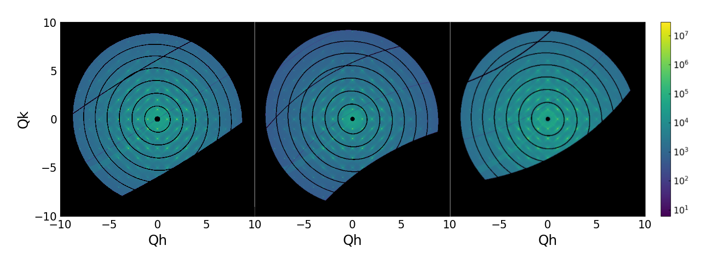
CCTW transforms from three rotation scans with detector translations.

Once all the rotation scans are processed, they are merged into a single reciprocal space grid.

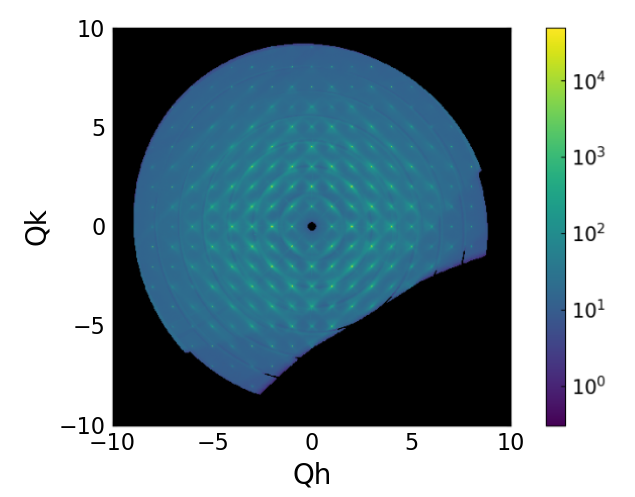
CCTW transform after merging the three rotation scans.

On a multi-core system, it is possible to accomplish the complete transformation process in less time than it takes to collect the data, even though the raw data can exceed 100 GB in size.