Python Interface to NeXus
The Python interface to NeXus is provided by the nexusformat package, which is distributed separately from NeXpy.
The Python API can be used within a standard Python or IPython shell:
% python
Python 3.13.5 | packaged by conda-forge | (main, Jun 16 2025, 08:23:50) [Clang 18.1.8 ] on darwin
Type "help", "copyright", "credits" or "license" for more information.
>>> from nexusformat.nexus import *
Note
Although wildcard imports are usually discouraged in Python, all the imported functions and variables start with ‘nx’ or ‘NX’, so the risk of namespace conflicts should be small.
See also
A Jupyter notebook provides a tutorial for the Python API. It can be run in Google Colaboratory.
Loading NeXus Data
The entire tree structure of a NeXus file can be loaded by a single command:
>>> root=nxload('data/GUP-75927-22-1/cno/bg_1/cno_30K.nxs')
The assigned variable now contains the entire tree structure of the file, which can be displayed by printing the ‘tree’ property:
>>> print(root.tree)
root:NXroot
 @HDF5_Version = '1.10.6'
 @default = 'f1'
 @file_name = '/net/s6iddata/export/s6buf1/GUP-75927-22-1/cno...'
 @file_time = '2022-03-18T19:30:16.169496'
 @h5py_version = '3.3.0'
 @nexusformat_version = '0.7.5.dev10+gf0406c7'
 entry:NXentry
 entry:NXentry
   @default = 'nxmasked_combine'
   instrument:NXinstrument
     detector:NXdetector
       description = 'Pilatus CdTe 2M'
       distance = 680.0
         @units = 'mm'
       frame_time = 0.1
         @units = 'second'
       pitch = 0.0
         @units = 'degree'
       pixel_mask = int8(1679x1475)
       pixel_size = 0.17200000000000001
         @units = 'mm'
       roll = 0.0
         @units = 'degree'
       shape = [1679 1475]
       yaw = 0.0
         @units = 'degree'
     monochromator:NXmonochromator
       energy = 86.72528557354696
         @units = 'keV'
       wavelength = 0.1429619938135147
         @units = 'angstrom'
   nxcombine:NXprocess
     @default = 'transform'
     date = '2022-03-22T16:22:12.851076'
 ...
Individual data items are immediately accessible from the command-line:
>>> print(root['entry/instrument/detector/distance'])
680.0
Only the tree structure and the values of smaller data sets are read from the file to avoid using up memory unnecessarily. In the above example, only the types and dimensions of the larger data sets are displayed in the tree. Data is loaded only when it is needed, for plotting or calculations, either as a complete array, if memory allows, or as a series of slabs (see below).
Note
The maximum size of data that will be read from a file into
memory can be configured using nxsetconfig. Details of
other configuration variables are described later.
There is a second optional argument to the load module that defines the access mode for the existing data. For example, the following opens the file in read/write mode:
>>> root=nxload('chopper.nxs', mode='rw')
The default mode is ‘r’, i.e., readonly access. The nxload function will accept any mode values allowed when opening h5py files, such as ‘r+’, ‘w’, ‘w-‘, and ‘a’ (see the h5py documentation for more details), but once open, the mode values are stored as ‘r’ or ‘rw’.
Warning
If the file is opened in read/write mode, any changes are
made automatically to the file itself. In particular, any
deletions of file objects will be irreversible. If
necessary, a backup of the file can be made using the
backup function.
See also
A context manager can be used to allow multiple read/write operations to be performed on the file before it is closed. Otherwise, the file is automatically opened and closed for each operation.
>>> with nxopen('nexus_file.nxs', 'w') as root:
>>>     root['entry'] = NXentry()
>>>     root['entry/sample'] = NXsample()
>>>     root['entry/sample/temperature'] = NXfield(40.0, units='K')
See also
nxopen is an alias for nxload. See Multiple
Operations for more details.
Creating NeXus Data
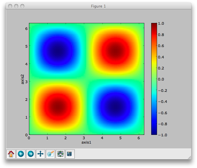
It is just as easy to create new NeXus data sets from scratch using NumPy arrays. The following example shows the creation of a simple function, which is then saved to a file:
>>> import numpy as np
>>> x=y=np.linspace(0,2*np.pi,101)
>>> X,Y=np.meshgrid(x,y)
>>> z=np.sin(X)*np.sin(Y)
>>> a=NXdata(z,[y,x])
>>> a.save('function.nxs')
This file can then be loaded again:
>>> b=nxload('function.nxs')
>>> print(b.tree)
root:NXroot
 @HDF5_Version = '1.14.6'
 @creator = 'nexusformat'
 @creator_version = '2.0.0'
 @file_name = '/home/user/function.nxs'
 @file_time = '2025-09-08T10:51:44.001605'
 @h5py_version = '3.13.0'
 entry:NXentry
   data:NXdata
     @axes = ['axis1', 'axis2']
     @signal = 'signal'
     axis1 = float64(101)
     axis2 = float64(101)
     signal = float64(101x101)
Note
The save() method automatically wraps any valid NeXus data in an NXentry group, in order to produce a standard-compliant file. See Saving NeXus Data for more details.
NeXus Objects
NeXus data are stored in a hierarchical tree structure, much like a computer file system. NeXus data structures consist of groups, with base class NXgroup, which can contain fields, with base class NXfield, and/or other groups.
NeXus Fields
NeXus data values are stored in NeXus objects of class ‘NXfield’. The NXfield class wraps standard NumPy arrays, scalars, and Python strings so that additional metadata (or attributes) and methods can be associated with them.
There are three ways to create an NXfield.
Direct assignment:
>>> x = NXfield(np.linspace(0,2*np.pi,101), units='degree')
The data value is given by the first positional argument, and may be a Python scalar or string, or a NumPy array. In this method, keyword arguments can be used to define NXfield attributes.
Dictionary assignment to the NeXus group:
>>> root['entry/sample/temperature']=40.0
Attribute assignment as the child of a NeXus group:
>>> root.entry.sample.temperature=40.0
The assigned values are automatically converted to an NXfield:
>>> root.entry.sample.temperature
NXfield(40.0)
Dictionary and attribute assignments are equivalent, but dictionary assignments should always be used if there is a danger of a name clash with, for example, group or field methods. They are also recommended when writing scripts. Attribute assignments are allowed because they are much faster to type in interactive sessions.
Note
When using the NeXpy GUI shell (see Python Graphical User Interface), it is possible to use tab completion to check for possible name clashes with NXfield methods. Autocompletion can be added as an extension to IPython sessions as well:
>>> from nexusformat.nexus.completer import load_ipython_extension
>>> load_ipython_extension(get_ipython())
The data in an NXfield can be of type integer, float, or character. The type is normally inherited automatically from the data type of the Python object, although it is possible to define alternative (but compatible) datatypes. For example, a float64 array can be converted to float32 on assignment:
>>> x=np.linspace(0, 2*np.pi,101)
>>> x.dtype
dtype('float64')
>>> a=NXfield(x, dtype='float32')
>>> a.dtype
dtype('float32')
>>> b=NXfield('Some Text')
>>> b.dtype, b.shape
(dtype('O'), ())
Note
Numeric dtypes can be defined either as a string, e.g., ‘int16’, ‘float32’, or using the NumPy dtypes, e.g., np.int16, np.float32.
Warning
By default, Python strings are stored as variable-length strings in the HDF5 file. These use a special object dtype defined by h5py (see the h5py documentation). If you wish to store fixed length strings, specify a dtype of kind ‘S’, e.g., ‘S10’ when creating the NXfield.
Warning
If you wish to store an array of strings containing Unicode characters as fixed-length strings, convert them to byte strings first using UTF-8 encoding, e.g.:
>>> text_array = ['a', 'b', 'c', 'd', 'é']
>>> a=NXfield([t.encode('utf8') for t in text_array], dtype='S')
>>> a
NXfield(['a', 'b', 'c', 'd', 'é'])
>>> a.dtype
dtype('S2')
The shape and dimension sizes of an integer or float array are inherited from the assigned NumPy array. It is possible to initialize an NXfield array without specifying the data values in advance, e.g., if the data is too large to be stored in memory and has to be written as slabs:
>>> a=NXfield(dtype=np.float32, shape=[2048,2048,2048])
>>> a
NXfield(shape=(2048, 2048, 2048), dtype=float32)
More details of handling large arrays are given below.
NeXus attributes
The NeXus standard allows additional attributes to be attached to NXfields to contain metadata
>>> root['entry/sample/temperature'].units='K'
These have a class of NXattr. They can be defined using the ‘attrs’ dictionary if necessary to avoid name clashes:
>>> root['entry/sample/temperature'].attrs['units']='K'
Other common attributes include the ‘signal’ and ‘axes’ attributes used to define the plottable signal and independent axes, respectively, in a NXdata group.
Note
The nxunits property of an NXfield can be used to read
and set units.
When a NeXus tree is printed, the attributes are prefixed by ‘@’:
>>> print(root['entry/sample'].tree)
sample:NXsample
  temperature = 40.0
    @units = 'K'
Masked Arrays
NumPy has the ability to store arrays with masks to remove missing or invalid data from computations of, e.g., averages or maxima. Since Matplotlib is able to handle masked arrays and removes masked data from plots, this is a convenient way of preventing bad data from contaminating statistical analyses, while preserving all the data values, good and bad, i.e., masks can be turned on and off.
NeXpy uses the same syntax as NumPy for masking and unmasking data.
>>> z = NXfield([1,2,3,4,5,6], name='z')
>>> z[3:5] = np.ma.masked
>>> z
NXfield(masked_array(data=[1, 2, 3, --, --, 6],
             mask=[False, False, False,  True,  True, False],
       fill_value=999999))
>>> z.mask
array([False, False, False,  True,  True, False])
>>> z.mask[3] = np.ma.nomask
>>> z
NXfield(masked_array(data=[1, 2, 3, 4, --, 6],
             mask=[False, False, False, False,  True, False],
       fill_value=999999))
Warning
If you perform any operations on a masked array, those operations are not performed on the masked values. It is not advisable to remove a mask if you have modified the unmasked values.
If the NXfield does not have a parent group, the mask is stored within the field as in NumPy arrays. However, if the NXfield has a parent group, the mask is stored in a separate NXfield that is generated automatically by the mask assignment or whenever the masked NXfield is assigned to a group. The mask is identified by the ‘mask’ attribute of the masked NXfield.
>>> print(NXlog(z).tree)
log:NXlog
z = [1 2 3 4 -- 6]
 @mask = 'z_mask'
z_mask = [False False False False  True False]
The mask can then be saved to the NeXus file if required.
Warning
In principle, the NXfield containing the mask can be modified manually, but it is recommended that modifications to the mask use the methods described above.
Masks can also be set using the Projection panel in the Python Graphical User Interface.
Large Arrays
If the size of an array is too large to be loaded into memory (see Loading NeXus Data), the NXfield can be created without any initial values, and then filled incrementally as slabs:
>>> entry['data/z'] = NXfield(shape=(1000,1000,1000), dtype=np.float32)
>>> for i in range(1000):
        entry.data.z[i,:,:] = np.ones(shape=(1000,1000), dtype=np.float32)
            ...
If entry in the above example is already stored in a NeXus file
(with write access), then entry['data/z'] is automatically updated
in the file. If it is not stored in a file, the field is stored in an
HDF5 core memory file that will be copied to the NeXus file when it is
saved.
When initializing the NXfield, it is possible to specify a number of HDF5 attributes that specify how the data are stored.
Compression:
>>> z = NXfield(shape=(1000,1000,1000), dtype=np.float32, compression='lzf')
This specifies the compression filter used. For large arrays, the data are compressed with the
gzipfilter by default.Chunk size:
>>> z = NXfield(shape=(1000,1000,1000), dtype=np.float32, chunks=(1,100,100))
By default, any field with more than 10000 elements will be initialized with
chunks=True. If chunk sizes are not specified, HDF5 will choose default values.Maximum array shape:
>>> z = NXfield(shape=(10,1000,1000), dtype=np.float32, maxshape=(1000,1000,1000))
The initial shape is defined by the
shapeattribute, but it will be automatically expanded up to a limit ofmaxshapeif necessary using the NXfieldresizefunction.>>> z.resize((100,1000,1000)) >>> z.shape (100, 1000, 1000)
Fill value:
>>> z = NXfield(shape=(1000,1000,1000), dtype=np.float32, fillvalue=np.nan)
Slabs that are not initialized will contain the specified fill value. This is normally set to zero by default.
All these values can be adjusted at the command line until the first
slab has been written, whether to a file or in core memory, using the
compression, chunks, maxshape or fillvalue properties,
e.g.,
>>> z = NXfield(shape=(1000,1000,1000), dtype=np.float32)
>>> z.compression = 'lzf'
Virtual Fields
Virtual fields contain data arrays assembled from entire arrays or slabs stored in multiple NeXus or HDF5 files. They are implemented as HDF5 virtual datasets, which contain pointers to the files and the paths within those files, so that the composite array can be treated as a single array for extracting slabs, e.g., for plotting.
In the nexusformat package, virtual fields are used to add an extra dimension to multidimensional fields stored in each file, whose size is equal to the number of files. If there is a scalar field that corresponds to a measurement parameter, such as temperature, that is changing in each file, a NXdata group can be created, using the nxconsolidate function, in which the parameter values define the axis of the extra dimension.
In the following example, each NeXus file contains a NXdata group with a
signal of shape (1000, 1000) and a scalar field containing the
temperature value. After creating the virtual field by combining all six
files, the resulting signal has a shape of (6, 1000, 1000). The
resulting NXdata group has temperature as an additional axis.
>>> scan_files = [f'scan_{T}K.nxs' for T in range(50, 300, 50)]
>>> data_path = '/entry/data'
>>> scan_path = '/entry/sample/temperature'
>>> with nxopen('scan.nxs', 'w') as root:
>>>     scan_data = nxconsolidate(scan_files, data_path, scan_path)
>>>     root['entry'] = NXentry(scan_data=scan_data)
>>> print(root['entry/scan_data'].tree)
scan_data:NXdata
 @axes = ['temperature', 'Qk', 'Qh']
 @signal = 'data'
 Qh = float64(1000)
 Qk = float64(1000)
 data = float64(6x1000x1000)
 temperature = float64(6)
>>> root['entry/scan_data'].nxsignal.__class__
nexusformat.nexus.tree.NXvirtualfield
Warning
The virtual field is initially stored in a HDF5 core memory file, but it should be saved to disk before further access. Mapping data in virtual fields to the original files is both slow and memory intensive using the HDF5 core driver.
NeXus Groups
NeXus groups are defined as subclasses of the NXgroup class, with the class name defining the type of information they contain, e.g., the NXsample class contains metadata that define the measured sample, such as its temperature or lattice parameters. The initialization parameters can be used to populate the group with other predefined NeXus objects, either groups or fields:
>>> temperature = NXfield(40.0, units='K')
>>> sample = NXsample(temperature=temperature)
>>> print(sample.tree)
sample:NXsample
  temperature = 40.0
    @units = 'K'
In this example, it was necessary to use the keyword form to add the NXfield ‘temperature’ since its name is otherwise undefined within the NXsample group. However, the name is set automatically if the NXfield is assigned to the group:
>>> sample = NXsample()
>>> sample['temperature']=NXfield(40.0, units='K')
>>> print(sample.tree)
sample:NXsample
  temperature = 40.0
    @units = 'K'
The NeXus objects in a group (NXfields or NXgroups) can be accessed as dictionary items:
>>> sample['temperature'] = 40.0
>>> sample.keys()
dict_keys(['temperature'])
Note
It is also possible to reference objects by their complete paths with respect to the root object, e.g., root[‘/entry/sample/temperature’].
If a group is not created as another group attribute, its internal name defaults to the class name without the ‘NX’ prefix. This can be useful in automatically creating nested groups:
>>> a=NXentry(NXsample(temperature=40.0),NXinstrument(NXdetector(distance=10.8)))
>>> print(a.tree)
entry:NXentry
  instrument:NXinstrument
    detector:NXdetector
      distance = 10.8
  sample:NXsample
    temperature = 40.0
See also
Existing NeXus objects can also be inserted directly into
groups. See nexusformat.nexus.tree.NXgroup.insert
NXdata Groups
NXdata groups contain data ready to be plotted. That means that the group should consist of an NXfield containing the signal and one or more NXfields containing the axes. NeXus defines a method of associating axes with the appropriate dimension, but NeXpy provides a simple constructor that implements this method automatically. This was already demonstrated in the example above, reproduced here:
>>> import numpy as np
>>> x=y=np.linspace(0,2*np.pi,101)
>>> X,Y=np.meshgrid(x,y)
>>> z=np.sin(X)*np.sin(Y)
>>> a=NXdata(z,[y,x])
The first positional argument is an NXfield or NumPy array containing the data, while the second is a list containing the axes, again as NXfields or NumPy arrays. In this example, the names of the arrays have not been defined within an NXfield so default names were assigned:
>>> print(a.tree)
data:NXdata
  @axes = ['axis1' 'axis2']
  @signal = signal
  axis1 = float64(101)
  axis2 = float64(101)
  signal = float64(101x101)
Note
The plottable signal and axes are identified by the ‘signal’ and ‘axes’ attributes of the NXdata group. The ‘axes’ attribute defines the axes as a list of NXfield names. The NXdata constructor sets these attributes automatically.
Warning
NumPy stores arrays by default in C, or row-major, order,
i.e., in the array ‘signal(axis1,axis2)’, axis2 is the
fastest to vary. In most image formats, e.g., TIFF
files, the x-axis is assumed to be the fastest varying
axis, so we are adopting the same convention and plotting
as signal[y,x]. The Python Graphical User Interface allows the x and
y axes to be swapped.
Names can be assigned explicitly when creating the NXfield through the ‘name’ attribute:
>>> phi=NXfield(np.linspace(0,2*np.pi,101), name='polar_angle')
>>> data=NXfield(np.sin(phi), name='intensity')
>>> a=NXdata(data,(phi,))
>>> print(a.tree)
data:NXdata
  @axes = 'polar_angle'
  @signal = 'intensity'
  intensity = float64(101)
  polar_angle = float64(101)
Note
In the above example, the x-axis, phi, was defined as a
tuple in the second positional argument of the NXdata call.
It could also have been defined as a list. However, in the
case of one-dimensional signals, it would also have been
acceptable just to call NXdata(data, phi), i.e.,
without embedding the axis in a tuple or list.
It is also possible to define the plottable signal and axes using the
nxsignal and nxaxes properties, respectively:
>>> phi=np.linspace(0,2*np.pi, 101)
>>> a=NXdata()
>>> a.nxsignal=NXfield(np.sin(phi), name='intensity')
>>> a.nxaxes=NXfield(phi, name='polar_angle')
>>> print(a.tree)
data:NXdata
  @axes = 'polar_angle'
  @signal = 'intensity'
  intensity = float64(101)
  polar_angle = float64(101)
Similarly, signal errors can be added using the nxerrors property:
>>> a.nxerrors = np.sqrt(np.abs(np.sin(phi)))
>>> print(a.tree)
data:NXdata
  @axes = 'polar_angle'
  @signal = 'intensity'
  intensity = float64(101)
  intensity_errors = float64(101)
  polar_angle = float64(101)
Note
In a NXdata group, errors for each field are defined by another field with ‘_errors’ appended to the name.
NeXus Links
NeXus allows groups and fields to be assigned to multiple locations
through the use of links. These objects have the class NXlink and
contain the attribute target, which identifies the parent object. It
is also possible to link to fields in another NeXus file (see External
Links below).
For example, the polar angle and time-of-flight arrays may logically be stored with the detector information in a NXdetector group that is one of the NXinstrument subgroups:
>>> print(entry['instrument'].tree)
instrument:NXinstrument
  detector:NXdetector
   distance = float32(128)
     @units = 'metre'
   polar_angle = float32(128)
     @units = 'radian'
   time_of_flight = float32(8252)
     @target = '/entry/instrument/detector/time_of_flight'
     @units = 'microsecond'
However, they may also be needed as plotting axes in a NXdata group:
>>> print(entry['data'].tree)
data:NXdata
  @axes = ['polar_angle' 'time_of_flight']
  @signal = data
  data = uint32(128x8251)
  polar_angle = float32(128)
    @target = '/entry/instrument/detector/polar_angle'
    @units = 'radian'
  time_of_flight = float32(8252)
    @target = '/entry/instrument/detector/time_of_flight'
    @units = 'microsecond'
Links allow the same data to be used in different contexts without using more memory or disk space.
Note
In earlier versions, links were required to have the same name as their parents, but this restriction has now been lifted.
In the Python API, the user who is only interested in accessing the data
does not need to worry if the object is parent or child. The data values
and NeXus attributes of the parent to the NXlink object can be accessed
directly through the child object. The parent object can be referenced
directly, if required, using the nxlink attribute:
>>> entry['data/time_of_flight']
NXlink('/entry/instrument/detector/time_of_flight')
>>> entry['data/time_of_flight'].nxdata
array([   500.,    502.,    504., ...,  16998.,  17000.,  17002.], dtype=float32)
>>> entry['data/time_of_flight'].units
'microsecond'
>>> entry['data/time_of_flight'].nxlink
NXfield(dtype=float32,shape=(8252,))
Note
The absolute path of the data with respect to the root object of the NeXus tree is given by the nxpath property:
>>> entry['data/time_of_flight'].nxpath
'/entry/data/time_of_flight'
>>> entry['data/time_of_flight'].nxlink.nxpath
'/entry/instrument/bank1/time_of_flight'
Creating a Link
Links can be created using the target object as the argument assigned to another group:
>>> print(root.tree)
root:NXroot
  entry:NXentry
    data:NXdata
    instrument:NXinstrument
      detector:NXdetector
        polar_angle = float64(192)
          @units = 'radian'
>>> root['entry/data/polar_angle']=NXlink(root['entry/instrument/detector/polar_angle'])
It is also possible to create links using the makelink method, which takes the parent object and, optionally, a new name as arguments:
>>> root['entry/data'].makelink(root['entry/instrument/detector/polar_angle'])
>>> print(root.tree)
root:NXroot
  entry:NXentry
    data:NXdata
      polar_angle = float64(192)
        @target = '/entry/instrument/detector/polar_angle'
        @units = 'radian'
    instrument:NXinstrument
      detector:NXdetector
        polar_angle = float64(192)
          @target = '/entry/instrument/detector/polar_angle'
          @units = 'radian'
Note
After creating the link, both the parent and target objects
have an additional attribute, target, showing the
absolute path of the parent.
External Links
It is also possible to link to a NeXus field that is stored in another file. This is accomplished using a similar syntax to internal links.
>>> root['entry/data/data'] = NXlink('/counts', file='external_counts.nxs')
In the case of external links, the first argument is the absolute path of the linked object within the external file, while the second argument is the absolute or relative file path of the external file.
By default, the target file path is converted to a relative path with
respect to the parent file. If it is required to store the absolute file
path, add the keyword argument, abspath=True.
>>> root['entry/data/data'] = NXlink('/counts',
                                 file='/home/user/external_counts.nxs',
                                 abspath=True)
Warning
If the files are moved without preserving their relative file paths, the parent file will still open but the link will be broken.
Modifying Links
The path to a linked object is given by the nxtarget property.
>>> root['entry/data/polar_angle'].nxtarget
'entry/instrument/detector/polar_angle'
If the link is external, nxtarget returns the object path within the
external file, whose file path is given by the nxfilename property.
>>> external_link = NXlink('/counts',
                           file='/home/user/external_counts.nxs')
>>> external_link.nxtarget
'/counts'
>>> external_link.nxfilename
'/home/user/external_counts.nxs'
HDF5 does not allow link targets to be changed, so the link has to be deleted and recreated. To facilitate this operation, nexusformat has added a setter function that allows the field path and/or file path to be modified (as long as the file is unlocked). If a single value is given, the object path is changed, provided that it points to a valid NeXus object.
If the link is external and nxtarget is a two-value tuple, the
values correspond to the object path in the external file and the file
path, respectively.
>>> external_link.nxtarget = ('/counts',
                              '/home/user/external_counts.nxs')
Plotting NeXus Data
NXdata, NXmonitor, and NXlog groups all have a plot method, which automatically determines what should be plotted:
>>> data.plot()
Note that the plot method uses the NeXus attributes within the groups to determine automatically which NXfield is the signal, what its rank and dimensions are, and which NXfields define the plottable axes. The same command will work for one-dimensional or two-dimensional data. If you plot higher-dimensional data, the top two-dimensional slice is plotted. Alternative two-dimensional slices can be specified using slice indices on the NXdata group.
Note
If the interpretation attribute is set to ‘rgb’ or ‘rgba’
and the final dimension is of size 3 or 4, the NXdata group
will be plotted as an image using the colors defined by the
final dimension. By default, images are displayed with the
origin in the top-left corner.
If the data is one-dimensional, it is possible to overplot more than one data set using ‘over=True’. By default, each plot has a new color, but conventional Matplotlib keywords can be used to change markers and colors:
>>> data.plot(log=True)
>>> data.plot('r-')
>>> data.plot(over=True, log=True, color='r')
If the NXdata group contains RGB(A) image data, i.e., the signal is a three-dimensional array, in which the fastest varying dimension, which should be of size 3 or 4, contains the RGB(A) values for each two-dimensional pixel, then the image can be plotted using the ‘image=True’.
>>> data.plot(image=True)
By convention, the first pixel of an image is in the upper-left corner, rather than the lower-left used in other two-dimensional plots.
Note
The plot method also works on NXroot and NXentry groups, if
they are able to identify plottable data. If the default
attribute is set, the default NXentry and/or NXdata groups
are used. Otherwise, the first valid NXdata group found in an
iterative search is used.
Additional Plot Methods
As a convenience, additional plot methods can be used instead of adding extra keywords.
>>> data.oplot()
>>> data.logplot()
>>> data.implot()
These are equivalent to setting the ‘over’, ‘log’, and ‘image’ keywords to True when invoking the plot method.
Manipulating NeXus Data
Arithmetic Operations
NXfield
NXfields usually consist of arrays of numeric data with associated metadata, the NeXus attributes (the exception is when they contain character strings). This makes them similar to NumPy arrays, and this module allows the use of NXfields in numerical operations as if they were NumPy ndarrays:
>>> x = NXfield((1.0,2.0,3.0,4.0))
>>> print(x+1)
[ 2.  3.  4.  5.]
>>> print(2*x)
[ 2.  4.  6.  8.]
>>> print(x/2)
[ 0.5  1.   1.5  2. ]
>>> print(x**2)
[  1.   4.   9.  16.]
>>> x.reshape((2,2))
NXfield([[ 1.  2.]
[ 3.  4.]])
>>> y = NXfield((0.5,1.5,2.5,3.5))
>>> x+y
NXfield(name=x,value=[ 1.5  3.5  5.5  7.5])
>>> x*y
NXfield(name=x,value=[  0.5   3.    7.5  14. ])
>>> (x+y).shape
(4,)
>>> (x+y).dtype
dtype('float64')
Such operations return valid NXfield objects containing the same attributes as the first NXobject in the expression. The ‘reshape’ and ‘transpose’ methods also return NXfield objects.
NXfields can be compared to other NXfields (this is a comparison of their NumPy arrays):
>>> y=NXfield(np.array((1.5,2.5,3.5)),name='y')
>>> x == y
True
NXfields are technically not a sub-class of the NumPy ndarray class,
but they are cast as NumPy arrays when required by NumPy operations,
returning either another NXfield or, in some cases, an array that can
easily be converted to an NXfield:
>>> x = NXfield((1.0,2.0,3.0,4.0))
>>> x.size
4
>>> x.sum()
10.0
>>> x.max()
4.0
>>> x.mean()
2.5
>>> x.var()
1.25
>>> x.reshape((2,2)).sum(1)
array([ 3.,  7.])
>>> np.sin(x)
array([ 0.84147098,  0.90929743,  0.14112001, -0.7568025 ])
>>> np.sqrt(x)
array([ 1.        ,  1.41421356,  1.73205081,  2.        ])
>>> print(NXdata(np.sin(x), (x)).tree)
data:NXdata
  @axes = 'x'
  @signal = 'signal'
  signal = [ 0.84147098  0.90929743  0.14112001 -0.7568025 ]
  x = [ 1.  2.  3.  4.]
Note
If a function will only accept a NumPy array, use the
nxvalue attribute, which returns the stored NumPy array.
>>> x.nxvalue
array([1., 2., 3., 4.])
NXdata Operations
Similar operations can also be performed on whole NXdata groups. If two NXdata groups are to be added, the rank and dimensions of the main signal array must match (although the names could be different):
>>> y=NXfield(np.sin(x),name='y')
>>> y
NXfield(name=y,value=[ 0.99749499  0.59847214 -0.35078323])
>>> a=NXdata(y,x)
>>> print(a.tree)
data:NXdata
  @axes = 'x'
  @signal = 'y'
  x = [ 1.5  2.5  3.5]
  y = [ 0.99749499  0.59847214 -0.35078323]
>>> print((a+1).tree)
data:NXdata
  @axes = 'x'
  @signal = 'y'
  x = [ 1.5  2.5  3.5]
  y = [ 1.99749499  1.59847214  0.64921677]
>>> print((2*a).tree)
data:NXdata
  @axes = 'x'
  @signal = 'y'
  x = [ 1.5  2.5  3.5]
  y = [ 1.99498997  1.19694429 -0.70156646]
>>> print((a+a).tree)
data:NXdata
  @axes = 'x'
  @signal = 'y'
  x = [ 1.5  2.5  3.5]
  y = [ 1.99498997  1.19694429 -0.70156646]
>>> print((a-a).tree)
data:NXdata
  @axes = 'x'
  @signal = 'y'
  x = [ 1.5  2.5  3.5]
  y = [ 0.  0.  0.]
>>> print((a/2).tree)
data:NXdata
  @axes = 'x'
  @signal = 'y'
  x = [ 1.5  2.5  3.5]
  y = [ 0.49874749  0.29923607 -0.17539161]
If data errors are included in the NXdata group, then the errors are propagated according to the operand:
>>> print(a.tree)
data:NXdata
  @axes = 'x'
  @signal = 'y'
  x = [ 1.5  2.5  3.5]
  y = [ 0.99749499  0.59847214  0.35078323]
  y_errors = [ 0.99874671  0.77360981  0.59226956]
>>> print((a+a).tree)
data:NXdata
  @axes = 'x'
  @signal = 'y'
  x = [ 1.5  2.5  3.5]
  y = [ 1.99498997  1.19694429  0.70156646]
  y_errors = [ 1.41244114  1.09404949  0.83759564]
Some statistical operations can be performed on the NXdata group.
NXdata.sum(axis=None):Returns the sum of the NXdata signal data. If the axis is not specifed, the total is returned. Otherwise, it is summed along the specified axis. The result is a new NXdata group containing a copy of all the metadata contained in the original NXdata group:
>>> x=np.linspace(0, 3., 4)
>>> y=np.linspace(0, 2., 3)
>>> X,Y=np.meshgrid(x,y)
>>> a=NXdata(X*Y,(y,x))
>>> print(a.tree)
data:NXdata
  @axes = ['axis1' 'axis2']
  @signal = 'signal'
  axis1 = [ 0.  1.  2.  3.]
  axis2 = [ 0.  1.  2.]
  signal = float64(3x4)
>>> a.nxsignal
NXfield([[ 0.  0.  0.  0.]
 [ 0.  1.  2.  3.]
 [ 0.  2.  4.  6.]])
>>> a.sum()
18.0
>>> a.sum(0).nxsignal
NXfield([ 0.  3.  6.  9.])
>>> a.sum(1).nxsignal
NXfield([  0.   6.  12.])
NXdata.average(axis=None):Returns the average of the NXdata signal data. This is identical to the sum method, but the result is divided by the number of data elements in the summation:
>>> a.average()
NXfield(1.5)
>>> a.average(0).nxsignal
NXfield([ 0.,  1.,  2.,  3.])
>>> a.average(1).nxsignal
NXfield([ 0. ,  1.5,  3. ])
NXdata.moment(order=1):Returns an NXfield containing the first moment of the NXdata group assuming the signal is one-dimensional:
>>> x=np.linspace(0, 10., 11)
>>> y=np.exp(-(x-3)**2)
>>> a=NXdata(y,x)
>>> a.moment()
NXfield(3.000000253977615)
Slicing
NXfields
A slice of an NXfield can be obtained using the usual Python indexing syntax:
>>> x=NXfield(np.linspace(0,2*np.pi,101))
>>> print(x[0:51])
[ 0.          0.06283185  0.12566371 ...,  3.01592895  3.0787608 3.14159265]
If either of the indices are floats, then the limits are set by the values themselves (assuming the array is monotonic):
>>> print(x[0.5:1.5])
[ 0.50265482  0.56548668  0.62831853 ...,  1.38230077  1.44513262 1.50796447]
NXdata
It is also possible to slice whole NXdata groups. In this case, the slicing works on the multidimensional NXfield, but the full NXdata group is returned with both the signal data and the associated axes limited by the slice parameters. If either of the limits along any one axis is a float, the limits are set by the values of the axis:
>>> a=NXdata(np.sin(x),x)
>>> a[1.5:2.5].x
NXfield(name=x,value=[ 1.57079633  1.72787596  1.88495559 ...,  2.19911486  2.35619449])
Unless the slice reduces one of the axes to a single item, the rank of the data remains the same. To project data along one of the axes, and so reduce the rank by one, the data can be summed along that axis using the sum() method. This employs the NumPy array sum() method:
>>> x=y=NXfield(np.linspace(0,2*np.pi,41))
>>> X,Y=np.meshgrid(x,y)
>>> a=NXdata(np.sin(X)*np.sin(Y), (y,x))
>>> print(a.tree)
data:NXdata
  @axes = ['axis1' 'axis2']
  @signal = 'signal'
  axis1 = float64(41)
  axis2 = float64(41)
  signal = float64(41x41)
>>> print(a.sum(0).tree)
data:NXdata
  @axes = 'axis2'
  @signal = 'signal'
  axis2 = float64(41)
  signal = float64(41)
    @long_name = 'Integral from 0.0 to 6.28318530718'
This can be extended to higher dimensions, using a tuple as the sum() argument. The following code projects a NXdata group, whose signal is a three-dimensional array, down to a one-dimensional NXdata group. The average values of the summed axes are stored as fields, with attributes showing the range of the summation.
>>> signal=NXfield(np.arange(60).reshape((3,4,5)), name='v')
>>> x=NXfield(np.arange(5.0), name='x')
>>> y=NXfield(np.arange(4.0), name='y')
>>> z=NXfield(np.arange(3.0), name='z')
>>> d=NXdata(signal, (z, y, x))
>>> print(d.tree)
data:NXdata
  @axes = ['z', 'y', 'x']
  @signal = 'v'
  v = int64(3x4x5)
  x = float64(5)
  y = float64(4)
  z = [0. 1. 2.]
>>> print(d.sum((0,1)).tree)
data:NXdata
  @axes = 'x'
  @signal = 'v'
  @summed_bins = 12
  title = 'data/data'
  v = int64(5)
  x = float64(5)
  y = 1.5
    @maximum = 3.0
    @minimum = 0.0
    @summed_bins = 4
  z = 1.0
    @maximum = 2.0
    @minimum = 0.0
    @summed_bins = 3
The Python Graphical User Interface provides a menu-based approach to simplify the plotting of 1D and 2D data projections of multidimensional data.
Saving NeXus Data
Every NeXus object, whether it is a group or a field, has a save() method as illustrated in Creating NeXus Data.:
>>> root.save(filename='example.nxs')
NXroot Groups
If the NeXus object is a NXroot group, the save() method saves the whole NeXus tree. The filename can only be omitted if the tree is being saved to a file that was loaded with read/write access. In this case, the format argument is ignored. If the tree was loaded with readonly access, any modifications must be saved to a new file specified by the filename argument.
Other Objects
If the object is not a NXroot group, a new file will be created containing the selected object and its children. A filename must be specified. Saving non-NXroot data allows parts of a NeXus tree to be saved for later use, e.g., to store an NXsample group that will be added to other files. The saved NeXus object is wrapped in an NXroot group and an NXentry group (with name ‘entry’), if necessary, in order to produce a valid NeXus file.
Validating NeXus Data
NeXus groups can be checked against the current definitions of the NeXus standard to look for non-compliant entries. The results are colorized, with errors printed in red, warnings printed in orange, and informational messages in black. Keyword arguments allow the results to be filtered, with only warnings and errors output by default.
NXgroup objects have the following methods.
- check():
This checks the contents of the NeXus group and its children against the base class definition.
>>> root['entry/sample'].check(errors=True)
- validate():
This validates a NXentry group against the application definition specified by the
definitionfield or against another file specified as a keyword argument. This checks that the fields and groups required by the application definition are included. This method can only be applied to NXentry, NXsubentry, and NXroot groups (in which the first entry is selected).>>> root['data'].validate(info=True)
- inspect():
This displays the base class definition as formatted XML.
>>> root['entry'].inspect(info=True)
Note
By default, the groups are compared against the NeXus
definition files contained within the package. Alternative
definitions my be defined, either by setting the path to the
definitions directory using `nxsetconfig(definitions="/path/
to/definitions")` or by defining the NX_DEFINITIONS
environment variable. The path should contain subdirectories
named ‘base_classes’, ‘applications’ and
‘contributed_definitions’.
Warning
These functions do not produce any output when run within the NeXpy shell. Please use the Validate Data menu item when using NeXpy.
NeXus File Operations
Changes to a NeXus tree that has been loaded from disk or saved to a file are automatically updated in the HDF5 file, assuming that it is opened with read/write permissions. This means that the tree is always an accurate representation of the current state of the NeXus file, unless it has been modified by an external process, in which case, the file should be reloaded.
Note
In the Python Graphical User Interface, the lock icon color for an externally modified file changes to red.
When a file is loaded, using the nxload function, the nxfile
attribute of the root group is an NXFile object, which is thin
wrapper over the underlying h5py.File object:
>>> root = nxload('chopper.nxs', 'r')
>>> root['entry']
NXentry('entry')
>>> root.nxfile['/entry']
<HDF5 group "/entry" (10 members)>
The nxload function can also be used to create a new file with the
mode set to ‘w’. Any keywords accepted by h5py.File can be used to
customize the new HDF5 file, e.g., to turn on SWMR mode.
Warning
There is usually no need to call the nxfile attribute
except to invoke the context manager (see next section).
If it is referenced, the underlying h5py.File object
is left open. It should be explicitly closed by calling
root.nxfile.close(). The current status of the file can be determined by calling root.nxfile.is_open().
Multiple operations
When a change is made to a NeXus file, which is open with read/write access, it is automatically opened, updated, and then closed to ensure that any changes are flushed to the file and other processes can read the file if necessary. When writing or modifying multiple items in the file, it is possible to use a context manager to prevent multiple open/close operations:
>>> with root.nxfile:
>>>     root['entry/sample'] = NXsample()
>>>     root['entry/sample/temperature'] = NXfield(40.0, units='K')
>>>     root['entry/sample/mass'] = NXfield(5.0, units='g')
The file will be opened at the start of the of the with clause and
closed automatically at the end.
Note
This context manager can be nested so it is safe to add a
with clause within a function that might, in some
implementations, be embedded in another with clause. The
file is only closed when the outermost context manager is
exited.
Alternatively, it is possible to use a context manager directly with
NXroot objects, rather than its associated NXfile.
This allows the use of a similar syntax to the Python open function,
in which a with clause ensuring that the file is opened and closed,
before and after the file access, respectively. To make this analogy
clearer, nxopen was added as an alias to nxload.
In the following code, a NeXus file is created, filled with NeXus objects and then closed.
>>> with nxopen('nexus_file.nxs', 'w') as root:
>>>     root['entry'] = NXentry()
>>>     root['entry/sample'] = NXsample()
>>>     root['entry/sample/temperature'] = NXfield(40.0, units='K')
File Locking
The context manager can also be used to lock the NeXus file to prevent other processes from accessing the file. According to the HDF5 documentation, concurrent read access is supported if the HDF5 library has been built as thread-safe. This appears to be the default with conda installations, for example. However, concurrent read and write access is only allowed when using SWMR mode. To prevent issues with multiple processes accessing the same file, nexusformat contains a simple file-locking mechanism, which is designed to work even when the processes are running on separate nodes and when other file-locking mechanisms might prove unreliable (e.g., on NFS-mounted disks).
Warning
Unfortunately, the word ‘lock’ can cause confusion because it is commonly used to refer to two different operations. The other one is to switch a file from read/write to read-only mode, e.g.,
>>> root.lock()
This operation will prevent the current process from writing to the file, but it does not add a file lock to prevent I/O conflicts with other processes.
A new file is created with the same name as the NeXus file, with the additional extension ‘.lock’. Other processes using the nexusformat package will wait until the lock is cleared before performing any further I/O operations. By default, this lock file is created in the same directory as the NeXus file, but this will fail if the user does not have sufficient permissions to create the file in that directory. For this reason, it is possible to define another directory with relaxed group and/or world permissions to store the lock files.
Configuring File Locks
File-locking is configured using nxgetconfig and nxsetconfig
(see next section). File locking is enabled by setting a non-zero value
for the lock parameter, which defines the length of time the process
will wait before triggering a NXLockException exception. Then, the
context manager described above will create and remove the lock file at
the beginning and end of the with clause, respectively.
>>> nxgetconfig('lock')
0
>>> nxsetconfig(lock=10)
>>> with root.nxfile:
>>>     root['entry/sample'] = NXsample()
>>>     root['entry/sample/temperature'] = NXfield(40.0, units='K')
The lock file name is the name of the NeXus file with .lock
appended. If a stale lock is encountered, it may be cleared by calling
clear_lock:
>>> root.nxfile.is_locked()
True
>>> root.nxfile.clear_lock()
>>> root.nxfile.is_locked()
False
Note
This lock is advisory. It is only guaranteed to work if the external process is also using nexusformat.
Serializing NeXus Data
NeXus groups and fields have functions that allow them to be serialized and deserialized for transmission over a network. The NeXus objects are converted into Python dictionaries, whose values can be used to reconstruct the original file using class methods.
>>> input_root = nxload('chopper.nxs')
>>> s = input_root.serialize()
>>> output_root = NXroot.deserialize(s)
Note
If the NeXus tree contains any external links, their respective files will have to be separately serialized. deserialized and saved to the same relative file location before the links will be resolved.
Configuration Parameters
The nexusformat package uses a number of parameters to configure its
default behavior. These are stored internally in a dictionary, which may
be read or modified using the nxgetconfig and nxsetconfig
functions, respectively.
>>> nxgetconfig()
{'compression': 'gzip',
 'definitions': None,
 'encoding': 'utf-8',
 'lock': 0,
 'lockexpiry': 28800,
 'lockdirectory': None,
 'maxsize': 10000,
 'memory': 2000,
 'recursive': False}
>>> nxsetconfig(memory=4000)
>>> nxgetconfig('memory')
4000
Here is a list of the current configuration parameters and their defaults.
compression:This sets the default HDF5 compression filter. The default is ‘gzip’.
definitions:This sets the path to the directory containing NeXus base class and application definitions. The default is None, in which case the definitions installed with the package are used.
encoding:This sets the default encoding for input strings. The default is ‘utf-8’.
lock:This sets the number of seconds before an attempted file lock acquisition times out. The default is 10 seconds. If set to 0, file locking is disabled (but see below).
lockexpiry:This sets the number of seconds before a file lock is considered stale. If the lock file is older than this value, a new lock can be acquired. The default is 28,800 seconds (8 hours).
lockdirectory:This defines the path to a directory, in which to store the lock files. The directory should be set to allow users to create files. The default is None, in which case, file locks are stored in the same directory as the NeXus file to be locked.
Note
If
lockdirectoryis defined, thelockparameter is automatically set to 10 seconds if the currently set value is 0, i.e., defining a lock directory is enough to enable file locking.
maxsize:This sets the maximum size of an array before HDF5 chunking and compression is turned on by default. The default is 10,000.
memory:This sets the memory limit (in MB) for loading arrays into memory. If a field contains data that is larger than this limit, it can only be accessed as a series of smaller slabs using the standard slicing syntax. The default is 2000 MB.
recursive:This sets the default method of loading NeXus files. If the value is set to True, all objects in the file are loaded (lazily) into memory. If set to False, only the first two levels of hierarchy are initially loaded. Lower levels are loaded when they are referenced. This includes tests for the existence of object paths in the file. The default is False.
Environment variables
The configuration parameters can also be set by defining environment variables, defined either in a user’s login files or by a system administrator. This is particularly useful for setting a system-wide lock-file directory for all users accessing the same data.
When the nexusformat package is loaded, environment variables take
precedence over the package defaults. The user can still override them
manually by calling nxsetconfig.
All of the configuration parameters defined in the previous section can
be defined. The equivalent environment variable name is constructed by
prefixing the parameter name in upper case by ‘NX_’, e.g.,
NX_COMPRESSION, NX_DEFINITIONS, NX_ENCODING, etc.